Course Notes:
A First Course on Numerical Methods by Uri M. Ascher and Chen Greif. These notes are provided for the private use of students enrolled in CPSC 303 at UBC in 2007-2008, and are not to be redistributed.
Additional Handouts:
| Date | Topic | Omitted |
|---|
Collaboration Policy:
You may collaborate with other students in the class on homework questions prior to writing up the version that you will submit. This collaboration may include pseudo-code solutions to programming components. Once you begin writing the version that you will submit, you may no longer collaborate on that question, either by discussing the solution with other students, showing your solution to other students, or looking at the solutions written by other students. Some additional prohibitions:
You may seek help from the course instructor or TA at any time while preparing your homework solutions. You may not receive help from any other person.
If you feel that you have broken this collaboration policy, you may cite in your homework solution the name of the person from whom you received help, and your grade will be suitably adjusted to take this collaboration into account. If you break this collaboration policy and fail to cite your collaborator, you will be charged with plagarism as outlined in the university calendar. If you have any questions, please contact the instructor.
More information is available from (among other sources):
Homework Submission Policy:
Homeworks:
| # | Topic | Assigned | Due Date | Max Late Days | Assignment | Other Assignment Files & Links | Solution | Other Solution Files & Links | Omitted |
|---|
Intended Audience: Undergraduates in
Prerequisites:
|
Instructor: Ian Mitchell
|
TA: Tin Yin (Philip) Lam
|
Course Communication:
Lectures: 12:00 - 13:00, Monday / Wednesday / Friday, Dempster 301
Grades: Your final grade will be based on a combination of:
Textbooks:
Other References:
| # | Date | Topic | Links | Required Readings | Optional Readings | Learning Goals |
|---|---|---|---|---|---|---|
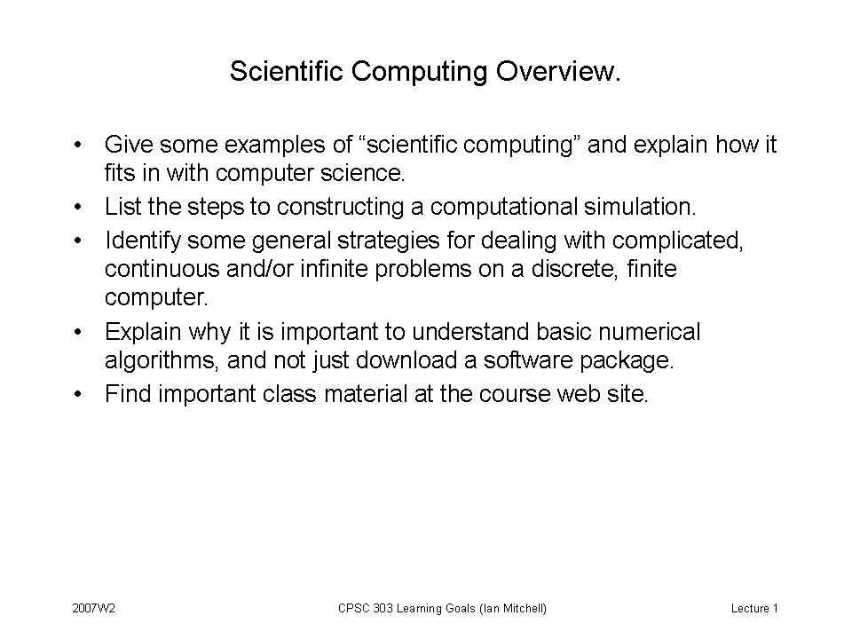
| 1 | Jan 7 | Introduction to Scientific Computing. | Scientific Computing overview slides. Matlab code for the Lorenz model: butterfly.m. | None. | H Preface; AG Preface; BF Preface | Goals |
| 2 | Jan 9 | Course Syllabus and Administration. Process of Simulation. | Nick Trefethen's essay on the definition of numerical analysis (pdf format), or get the original (ps format). | H 1.1-1.2; AG 1.1 | H 1.4-1.5 | Goals |
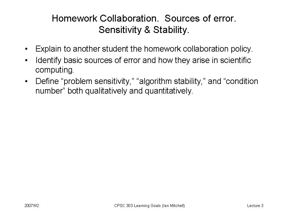
| 3 | Jan 11 | Collaboration guidelines. Sources (Types) of Error. Problem sensitivity and Algorithm Stability. Measures of Error: Absolute & Relative. | None. | H 1.2; AG 1.2 | AG 1.3; BF 1.3 | Goals |
| 4 | Jan 14 | Methods of Analyzing Error: Forward and Backward. Floating Point Properties. | Interactive Education Module on Floating Point Arithmetic. An interview William Kahan, "father" of IEEE floating point. Kahan's lecture notes on IEEE 754 | H 1.3; AG 2.0, 2.1, 2.3 | BF 1.2 | Goals |
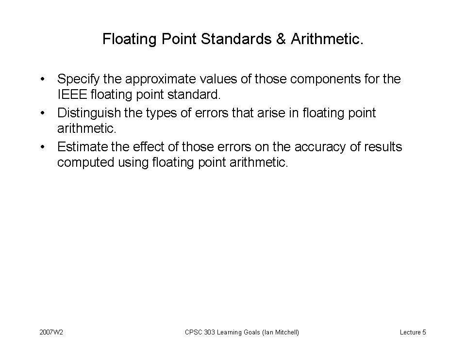
| 5 | Jan 16 | Floating Point Standard and Arithmetic. | None. | H 1.3; AG 2.2, 2.4 | None. | Goals |
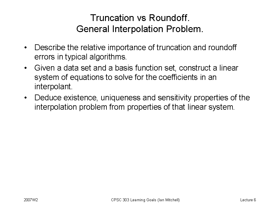
| 6 | Jan 18 | Sources (Types) of Error during Computation: Truncation and Rounding. Interpolation: Background, Problem Formulation. | An example of polynomial interpolation in Matlab: interpolateSine.m | H 7.0-7.3.0; AG 11.0 | BF 3.0 | Goals |
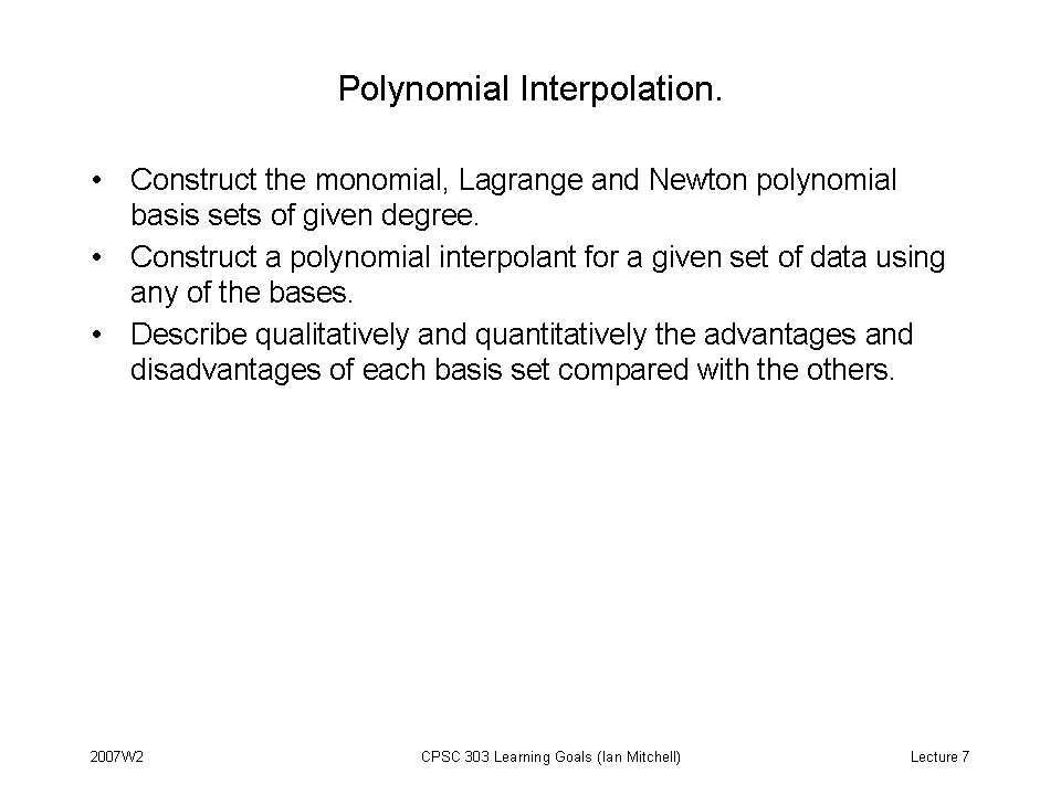
| 7 | Jan 21 | Monomial Basis. Lagrange Basis. | Interactive Education Modules for showing the polynomial bases and showing some interpolants in various bases. | H 7.3.1-7.3.3; AG 11.1-11.3 | BF 3.1-3.2 | Goals |
| 8 | Jan 23 | Newton Basis. | Interactive Education Module for constructing the Newton interpolant point by point. There are several other modules under interpolation covering topics that we will not get to in class. | AG 11.3 | AG 11.7; BF 3.2 | Goals |
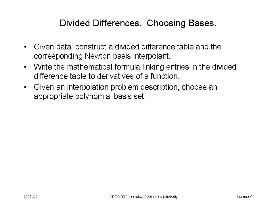
| 9 | Jan 25 | Divided Differences. Choosing Polynomial Bases. | None. | None. | None. | Goals |
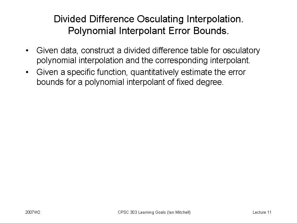
| 10 | Jan 28 | Another Divided Difference Table. Osculating (or Hermite) Interpolation. | None. | H 7.4.1; AG 11.5 | BF 3.3 | Goals |
| 11 | Jan 30 | Interpolation Error | interpolateRunge.m and the handout with Interpolation Error examples. Interactive Education Modules for polynomial interpolant error bounds and convergence of the interpolant as n increases. | H 7.3.5; AG 11.4 | H 7.3.4; AG 11.7, 13.4; BF 8.3 | Goals |
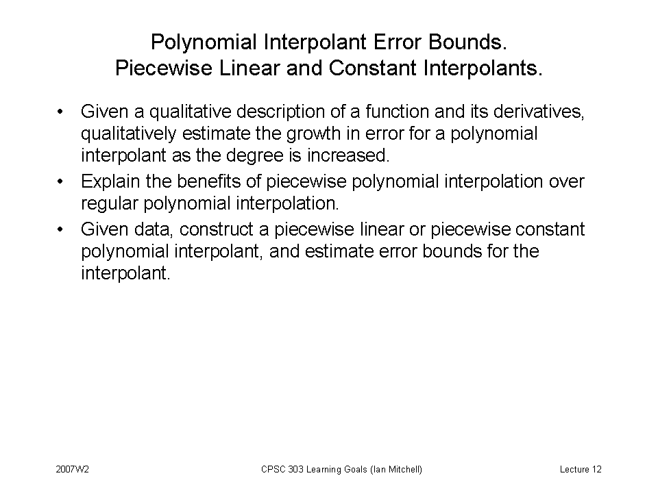
| 12 | Feb 1 | Piecewise Polynomial Interpolation. | None. | H 7.4.0; AG 12.0-12.1 | BF 3.4 | Goals |
| 13 | Feb 4 | Higher degree piecewise polynomial interpolants. | Slides showing the equations that various types of interpolants must satisfy. | AG 12.1 | None. | Goals |
| 14 | Feb 6 | Cubic Splines. Piecewise Hermite. | Piecewise Cubic example and the code piecewiseCubic.m. Interactive Education Modules for piecewise cubic interpolation and comparing basic polynomial interpolation with splines. | H 7.4.1-7.4.2; AG 12.2 | H 7.5-7.6; AG 12.7; BF 3.6 | Goals |
| Feb 8 | Midterm 1. | |||||
| 15 | Feb 11 | B-splines. | Online B-spline descriptions: Wikipedia or Mathworld. | H 7.4.3; AG 12.3; | None. | Goals |
| 16 | Feb 13 | More B-splines. | Example code: bsplineBasis.m evaluates bspline basis functions, bsplinePlot.m shows bspline basis sets of a specific degree for a given set of knots, and bsplineRunge.m demonstrates fitting a cubic spline to Runge's function using the cubic bspline basis set. | None. | None. | Goals |
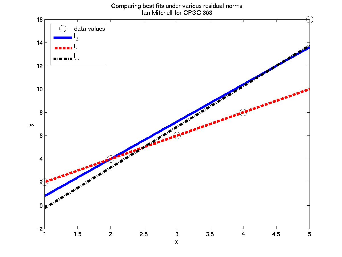
| 17 | Feb 15 | Parametric Interpolation. Best Approximation: Problem Formulation. | Example parametric.m of parametric interpolation of the slinky data. bestFitNormChoice.m computes the best linear fit under various norms for the data from class. Results | AG 12.4, 6.0 | H 3.2; BF 3.5, 8.1 | Goals |
| Feb 18-22 | Midterm Break. | |||||
| 18 | Feb 25 | Discrete Least Squares Data Fitting. | Discrete Least Squares example and the code lsDiscrete.m. Interactive Education Module for least squares data fitting. | AG 6.1; H 3.1, 3.4.1 | AG 6.2-6.3; H 3.3 (or even H 3) | Goals |
| 19 | Feb 27 | Numerical Differentiation. Symbolic & Automatic Differentiation. Taylor Series Methods. | None. | AG 15.0 - 15.1; H 8.6 | BF 4.1 | Goals |
| 20 | Feb 29 | Interpolate & Differentiate. Lagrange Basis Formulae. | Interactive Education Module for numerical differentiation. | AG 15.2; H 8.6 | AG 15.6; H 8.8, 8.9 | Goals |
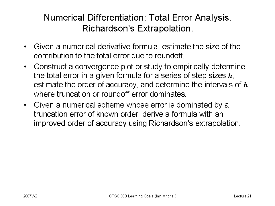
| 21 | March 3 | Errors in Numerical Differentiation. Richardson Extrapolation. | Richardson's Extrapolation example and the code richardson.m. Interactive Education Module for Richardson extrapolation. | AG 15.3-15.4; H 8.7 | BF 4.2 | Goals |
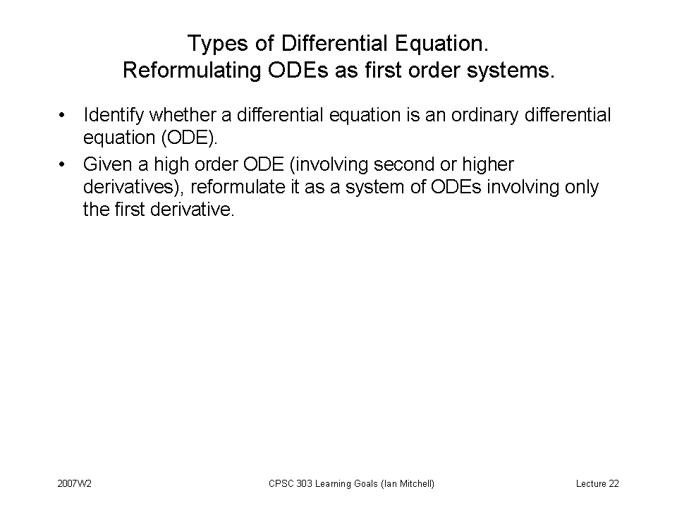
| 22 | March 5 | ODEs: introduction, high order reformulation. Lipschitz continuity. | Interactive Education Modules for ODE applications: predator-prey and epidemic progression. | AG 17.0; H 9.1 | BF 5.1, 5.9 | Goals |
| 23 | March 7 | ODE existence, uniqueness & conditioning. ODE Basic Methods: Forward Euler. | Example codes: pendulum.m, stiff.m, circle.m, and matlabFailure.m. For more information, see the ODE links below. | H 9.2 | BF 5.2 | Goals |
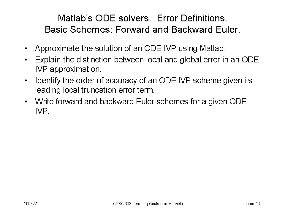
| 24 | March 10 | Integrator Error Analysis. Backward Euler. | Interactive Education Modules: forward Euler (also shows local vs global error) and backward Euler. | AG 17.1; H 9.3.1-9.3.3 | None. | Goals |
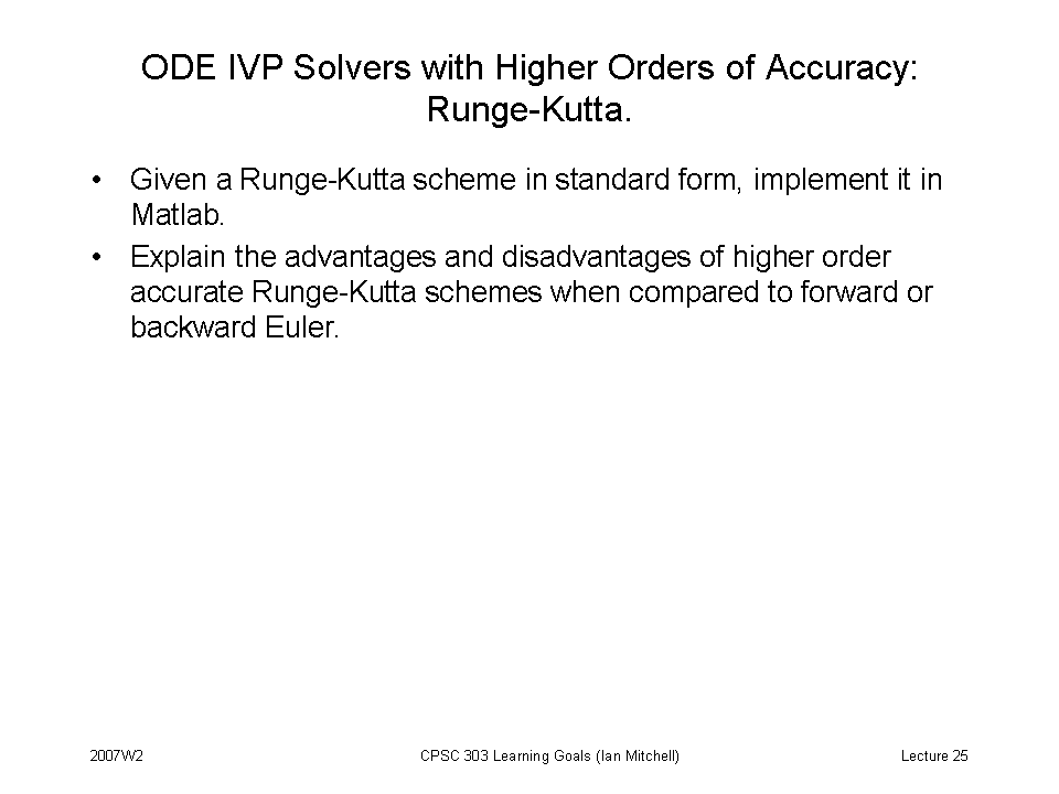
| 25 | March 12 | Higher Order Accuracy: Runge-Kutta Methods, including Implicit Trapezoidal & Explicit Midpoint. | Interactive Education Modules: implicit trapezoidal and Runge-Kutta (3 step). | AG 17.2; H 9.3.6 | BF 5.4 | Goals |
| March 14 | Midterm 2. | |||||
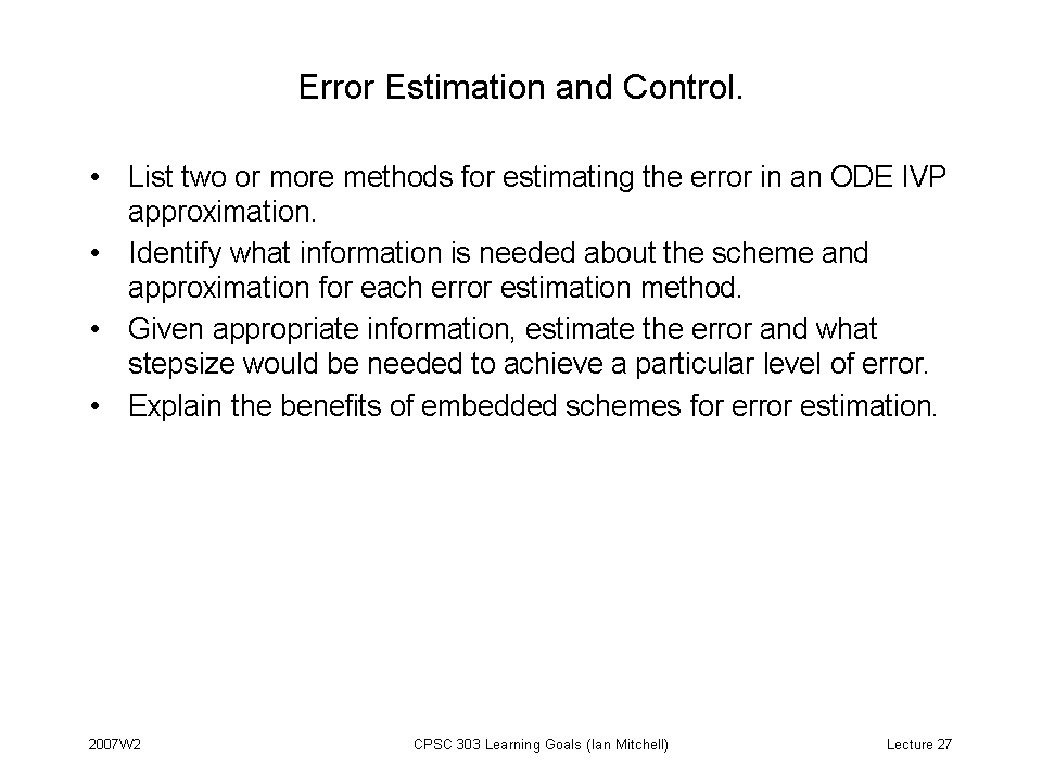
| 26 | March 17 | Higher Order Accuracy: Other Options. Error Estimation and Control. | Interactive Education Module: error estimation (uses y'' approximation; not recommended). | AG 17.3-17.4; H 9.3.5, 9.3.7-9.3.9 | BF 5.5 | Goals |
| 27 | March 19 | Embedded Schemes and Adaptive Stepsize Control. | astronomy.m demonstrates the benefits of adaptive stepsize error control (you will also need astroODE.m and rk4.m). | None. | None. | Goals |
| March 21 & 24 | Good Friday & Easter Monday. University Holidays. | |||||
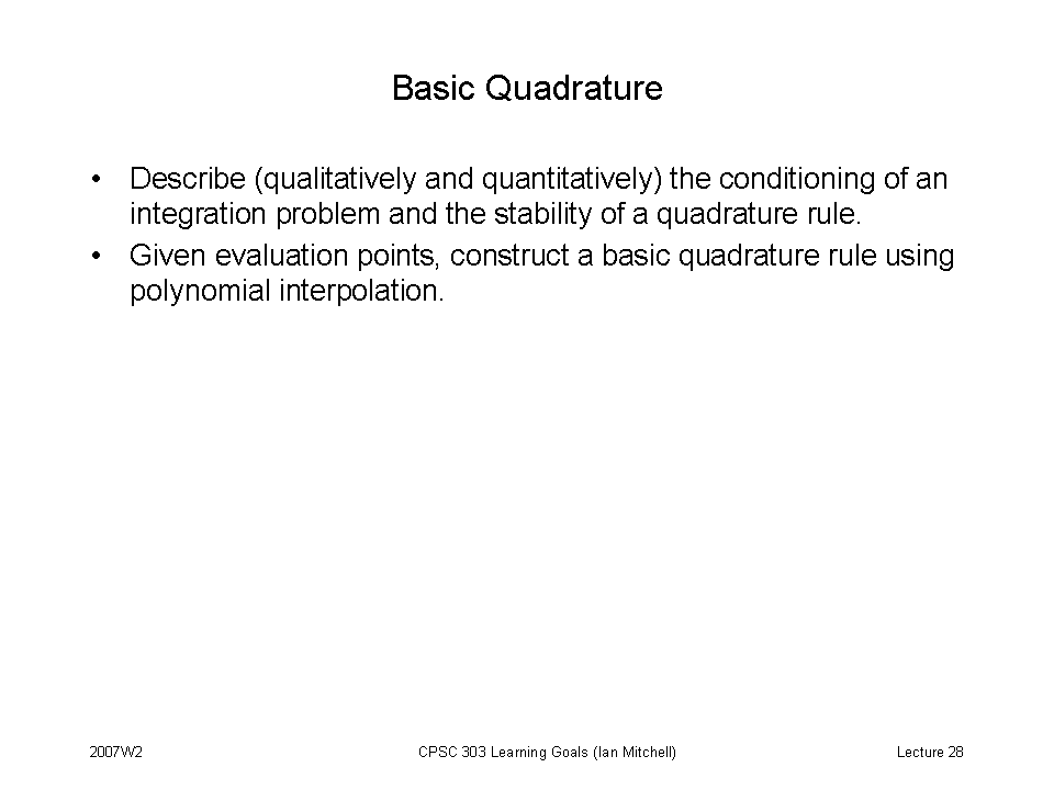
| 28 | March 26 | Introduction to Numerical Integration. Basic Quadrature. Guest Lecturer Michael Friedlander. | Interactive Education Modules: Newton-Cotes quadrature and cancellation of errors (why odd order Newton-Coates rules have greater precision than one might expect). | AG 16.0 - 16.1; H 8.1-8.3.2 | BF 4.3 | Goals |
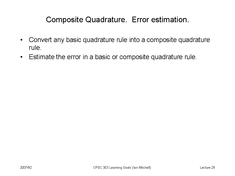
| 29 | March 28 | Composite Quadrature. Guest Lecturer Chen Greif. | None. | AG 16.2; H 8.3.5 | BF 4.4 | Goals |
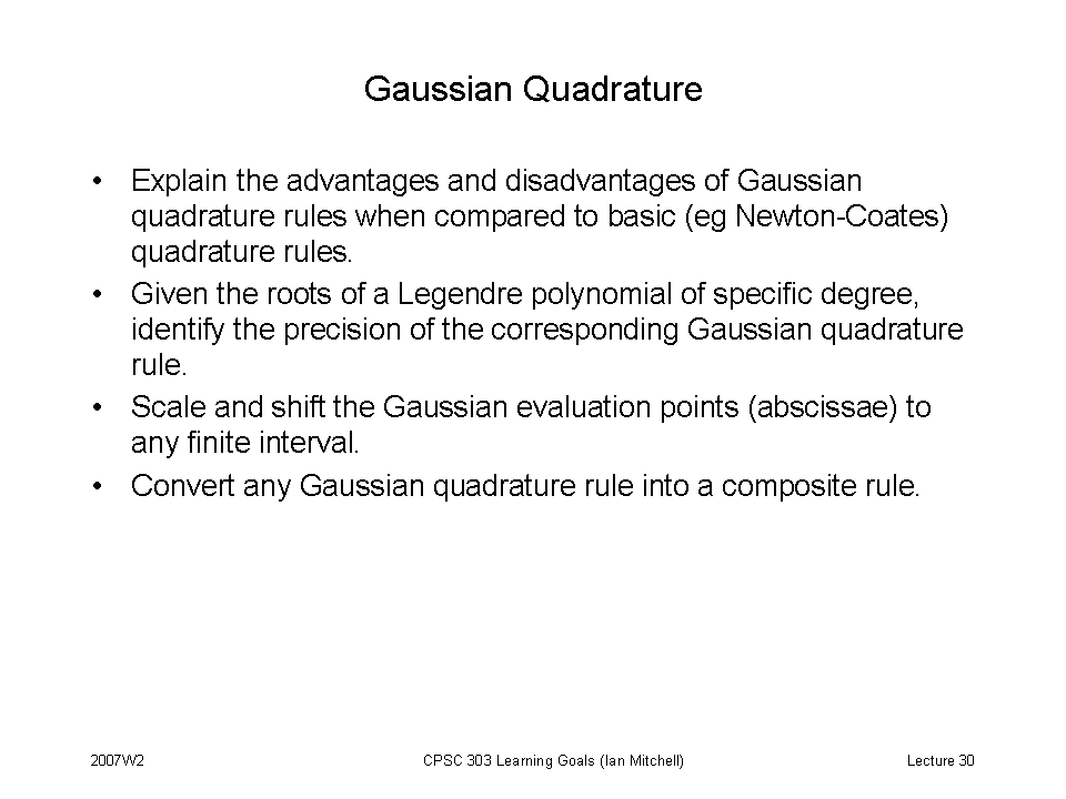
| 30 | March 31 | Gaussian Quadrature. | None. | AG 16.3, 16.4; H 8.3.3-8.3.4 | BF 4.7 | Goals |
| 31 | April 2 | Adaptive Quadrature. Quadrature wrap-up. | Interactive Education Module: adaptive quadrature. | AG 16.4; H 8.3.6 | AG 16.5-16.8; H 8.8-8.9; BF 4.6 | Goals |
| 32 | April 4 | ODE Stability. | None. | AG 17.5; H 9.3.2 | BF 5.10 | Goals |
| 33 | April 7 | ODE Stiffness & Stability. | stiff.m demonstrates a stiff system. Interactive Education Module: comparing forward and backward Euler for a stiff ODE. | AG 17.5; H 9.3.2-9.3.4 | BF 5.10 | Goals |
| 34 | April 9 | ODE Stiffness & Stability (continued). | None. | None. | AG 17.7; H 9.4-9.5; BF 5.11 | Goals |
| 35 | April 11 | Catchup Lecture. | None. | None. | None. | Goals |
| April 15-29 | Final Exam: Tuesday April 22, 15:30, DMP 201. | |||||