[Angel p267-290; Foley p721-741, 760-766]

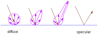
Traditional graphics LIMs are:
Most such adhoc illumination models have three components:
I = ambient + diffuse + specular
The ambient term allows for some global control of brightness in a scene. Typically,
I = Ia ka
where Ia is an ambient illumination constant defined once for the entire scene, and ka is an ambient reflection coefficient, usually restricted to lie in [0,1].

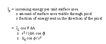
Id = Ii k_diff cos(th), th in [-pi/2, pi/2]
    = Ii k_diff (N.L),   N.L  0 and assuming N and L are          normalized
Ii: intensity of light source i
k_diff: surface reflection coefficient
th: angle between N and L
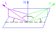
The last component of the commonly-used local illumination model is one that takes into account specular reflections. The following figure illustrates the situation:
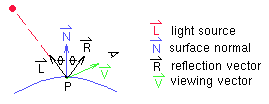
The Phong illumination model is one often-used method of calculating the specular component:
  Is = Ii k_spec cos^n(alpha)
     = Ii K_spec (R.V)^n
where k_spec is a specular reflection coefficient and alpha is the angle between the reflection and viewing vector. The surface parameter 'n' can be thought of as describing the surface roughness, where an ideal mirror would have n=¥ , and a rough surface might have n=1.
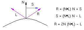
How can R be computed?
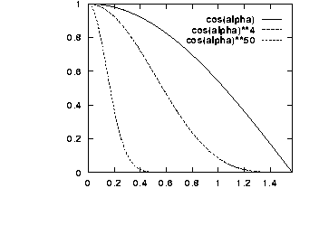
The function cos^n(alpha) looks as follows:
Blinn reformulated the specular reflection model so that it agreed better with experimental results. It makes use of a halfway vector, H, as follows:
Is = Ii k_spec cos^n(alpha)
     = Ii K_spec (N.H)^n
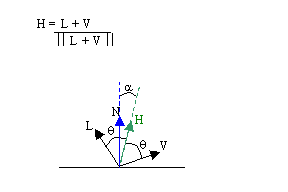 The advantages of this model include:
Combining the various models and assuming the Phong illumination model gives:
I = Ia ka + Ii k_diff (N.L) + Ii k_spec (R.V)^n
where each of ka, k_diff, and k_spec are parameters which are associated with specific surfaces and take on values between 0 and 1. To deal with colour, three equations of the above form are typically used:
I_r = Ia_r ka_r + Ii_r k_diff_r (N.L) + Ii_r k_spec_r (R.V)^n
I_g = Ia_g ka_g + Ii_g k_diff_g (N.L) + Ii_g k_spec_g (R.V)^n
I_b = Ia_b ka_b + Ii_b k_diff_b (N.L) + Ii_b k_spec_b (R.V)^n
Some other problems and their adhoc solutions:
The following are calls which set the parameters of a light:
  glLightfv(GL_LIGHT0, GL_AMBIENT, amb_light_rgba );
  glLightfv(GL_LIGHT0, GL_DIFFUSE, dif_light_rgba );
  glLightfv(GL_LIGHT0, GL_SPECULAR, spec_light_rgba );
  glLightfv(GL_LIGHT0, GL_POSITION, position);
  glEnable(GL_LIGHT0);
The following calls define the surface properties to be used for all subsequently drawn objects.
  glMaterialfv( GL_FRONT, GL_AMBIENT, ambient_rgba );
  glMaterialfv( GL_FRONT, GL_DIFFUSE, diffuse_rgba );
  glMaterialfv( GL_FRONT, GL_SPECULAR, specular_rgba );
  glMaterialfv( GL_FRONT, GL_SHININESS, n );
